XGBoost Training Time of Max Depth vs Boosting Rounds

When tuning XGBoost models, max_depth and n_estimators are two critical hyperparameters that significantly impact model performance and training time. In this example, we’ll explore how these parameters affect the training time of XGBoost models using a synthetic dataset.

We’ll generate a binary classification dataset and train XGBoost models with varying max_depth and n_estimators values. By measuring the training time for each combination, we can gain insights into how these parameters influence computational efficiency.

Finally, we’ll create a line plot to visualize the relationship between max_depth, n_estimators, and training time, enabling us to make informed decisions when tuning XGBoost models.

import time
import numpy as np
import pandas as pd
from sklearn.datasets import make_classification
from xgboost import XGBClassifier
import matplotlib.pyplot as plt

# Generate a synthetic dataset for binary classification
X, y = make_classification(n_samples=100000, n_features=20, n_informative=10, n_redundant=5, random_state=42)

# Define the range of max_depth and n_estimators values to test
max_depth_values = [1, 3, 5, 7, 9]
estimators_range = [50, 100, 200, 300, 400, 500]

# Initialize a DataFrame to store the results
results_df = pd.DataFrame(columns=['max_depth', 'estimators', 'training_time'])

# Iterate over the max_depth and n_estimators values
for depth in max_depth_values:
    for estimators in estimators_range:
        # Initialize an XGBClassifier with the specified parameters
        model = XGBClassifier(max_depth=depth, n_estimators=estimators, random_state=42)

        # Train the model and record the training time
        start_time = time.perf_counter()
        model.fit(X, y)
        end_time = time.perf_counter()
        training_time = end_time - start_time

        result = pd.DataFrame([{
            'max_depth': depth,
            'estimators': estimators,
            'training_time': training_time
        }])

        # Report progress
        print(result)

        # Append the results to the DataFrame
        results_df = pd.concat([results_df, result], ignore_index=True)

# Pivot the DataFrame to create a matrix suitable for plotting
plot_df = results_df.pivot(index='estimators', columns='max_depth', values='training_time')

# Create a line plot
plt.figure(figsize=(10, 6))
for depth in max_depth_values:
    plt.plot(plot_df.index, plot_df[depth], marker='o', label=f'max_depth={depth}')

plt.xlabel('Number of Estimators')
plt.ylabel('Training Time (seconds)')
plt.title('XGBoost Training Time vs. Number of Estimators and Max Depth')
plt.legend(title='Max Depth')
plt.grid(True)
plt.xticks(estimators_range)
plt.show()

The plot may look something like the following:

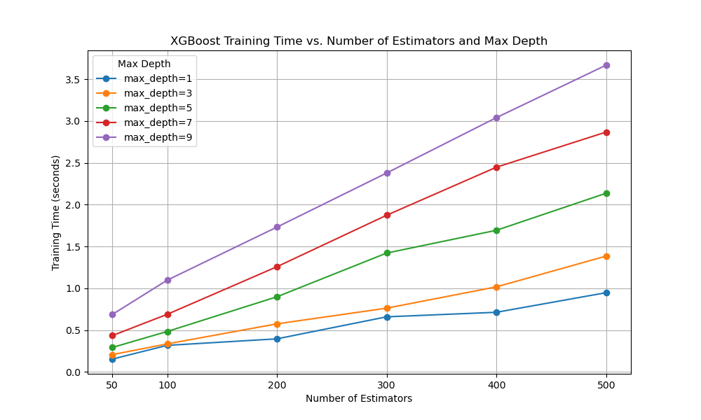
The resulting plot will display the training times for each max_depth value as the number of estimators increases. This allows us to understand how the training time scales with both max_depth and n_estimators.

From the plot, we can observe that:

• Increasing max_depth generally leads to longer training times, as the trees become more complex and require more computation.
• Training time increases linearly with n_estimators, as more trees are added to the ensemble.
• The impact of max_depth on training time becomes more pronounced as n_estimators increases.

When tuning XGBoost models, consider the trade-off between model performance and training time. While deeper trees and more estimators can improve model accuracy, they also require more computational resources and longer training times.

By visualizing the relationship between max_depth, n_estimators, and training time, you can make informed decisions based on your specific requirements and constraints. If training time is a critical factor, you may opt for shallower trees or fewer estimators, while still aiming to maintain acceptable model performance.

Remember that the optimal values for these hyperparameters may vary depending on the characteristics of your dataset and the computational resources available. Experiment with different combinations and monitor both model performance and training time to find the best balance for your use case.