
XGBoost is renowned for its speed and efficiency, and one of the ways it achieves this is through support for multithreading.
By utilizing multiple CPU cores, you can significantly reduce the time it takes to train your XGBoost models.
But how exactly does the number of threads affect training time, and how does this interact with other parameters like the number of estimators?
In this example, we’ll benchmark XGBoost’s training time while varying the number of threads (n_jobs) and the number of estimators (n_estimators).
We’ll use a synthetic dataset for binary classification and measure the training time for each combination of parameters. Finally, we’ll visualize the results as a line plot to help us understand the relationship between threads, estimators, and training time.
import os
import time
import numpy as np
import pandas as pd
from sklearn.datasets import make_classification
from xgboost import XGBClassifier
import matplotlib.pyplot as plt
# Generate a synthetic dataset for binary classification
X, y = make_classification(n_samples=10000, n_features=20, n_informative=10, n_redundant=5, random_state=42)
# Define the range of threads and estimators to test
threads_range = range(1, 5)
estimators_range = [10, 50, 100, 200, 300, 400, 500]
# Initialize a DataFrame to store the results
results_df = pd.DataFrame(columns=['threads', 'estimators', 'training_time'])
# Iterate over the number of threads and estimators
for threads in threads_range:
for estimators in estimators_range:
# Initialize an XGBClassifier with the specified parameters
model = XGBClassifier(n_jobs=threads, n_estimators=estimators, random_state=42)
# Train the model and record the training time
start_time = time.perf_counter()
model.fit(X, y)
end_time = time.perf_counter()
training_time = end_time - start_time
result = pd.DataFrame([{
'threads': threads,
'estimators': estimators,
'training_time': training_time
}])
# Report progress
print(result)
# Append the results to the DataFrame
results_df = pd.concat([results_df, result], ignore_index=True)
# Pivot the DataFrame to create a matrix suitable for plotting
plot_df = results_df.pivot(index='estimators', columns='threads', values='training_time')
# Create a line plot
plt.figure(figsize=(10, 6))
for threads in threads_range:
plt.plot(plot_df.index, plot_df[threads], marker='o', label=f'{threads} threads')
plt.xlabel('Number of Estimators')
plt.ylabel('Training Time (seconds)')
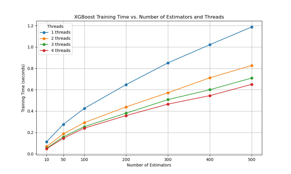
plt.title('XGBoost Training Time vs. Number of Estimators and Threads')
plt.legend(title='Threads')
plt.grid(True)
plt.xticks(estimators_range)
plt.show()
The plot captures the increase in training time as the number of boosting rounds is increased, and how these curves can be reduced by increasing the number of parallel threads used during training.
We can see that there is diminishing returns in terms of the number of threads used during training and the speed-up they offer.
The plot may look something like the following:
This example demonstrates how to benchmark XGBoost’s training time while varying the number of threads and estimators.
By visualizing the results as a line plot, you can gain insights into how these parameters affect training time and make informed decisions when tuning your XGBoost models for optimal performance.