XGBoost Plot Validation Curve

Validation curves are a powerful tool for evaluating the impact of individual hyperparameters on the performance of a machine learning model.

By plotting the model’s performance against different values of a specific hyperparameter, you can identify the optimal value that maximizes the model’s performance on unseen data.

his is particularly useful when working with complex models like XGBoost, which have many hyperparameters that can significantly influence the model’s behavior.

In this example, we’ll demonstrate how to use scikit-learn’s validation_curve function to plot validation curves for XGBoost’s max_depth hyperparameter, which controls the maximum depth of the decision trees in the ensemble.

import numpy as np
from sklearn.model_selection import validation_curve
from xgboost import XGBClassifier
from sklearn.datasets import make_classification
import matplotlib.pyplot as plt

# Generate synthetic binary classification dataset
X, y = make_classification(n_samples=1000, n_classes=2, random_state=42)

# Define XGBoost model
xgb_clf = XGBClassifier(n_estimators=100, random_state=42)

# Define range of values for max_depth
param_range = np.arange(1, 11)

# Calculate validation curves
train_scores, test_scores = validation_curve(
    estimator=xgb_clf, X=X, y=y, param_name="max_depth",
    param_range=param_range, cv=5, scoring="accuracy", n_jobs=-1)

# Calculate mean and standard deviation of scores
train_mean = np.mean(train_scores, axis=1)
train_std = np.std(train_scores, axis=1)
test_mean = np.mean(test_scores, axis=1)
test_std = np.std(test_scores, axis=1)

# Plot validation curves
plt.figure(figsize=(8, 6))
plt.plot(param_range, train_mean, color="blue", marker="o", label="Training score")
plt.fill_between(param_range, train_mean + train_std, train_mean - train_std, alpha=0.15, color="blue")
plt.plot(param_range, test_mean, color="green", marker="o", label="Validation score")
plt.fill_between(param_range, test_mean + test_std, test_mean - test_std, alpha=0.15, color="green")
plt.title("Validation Curves for XGBoost's max_depth")
plt.xlabel("max_depth")
plt.ylabel("Accuracy")
plt.grid()
plt.legend(loc="lower right")
plt.show()

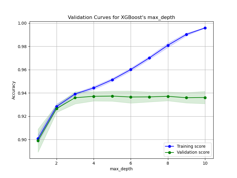
The generated plot may look like the following:

Let’s break down the code step by step:

1. We generate a synthetic binary classification dataset using scikit-learn’s make_classification function. In practice, you would use your actual training data.

2. We define an XGBoost classifier (XGBClassifier) with a fixed random state for reproducibility.

3. We define the range of values for the max_depth hyperparameter that we want to evaluate. In this case, we consider values from 1 to 10.

4. We use scikit-learn’s validation_curve function to calculate the training and validation scores for each value of max_depth. We specify the model, the dataset (X and y), the hyperparameter name and range, the number of cross-validation splits (cv=5), and the performance metric (scoring="accuracy").

5. The validation_curve function returns the training and validation scores for each value of max_depth. We calculate the mean and standard deviation of these scores across the cross-validation splits.

6. Finally, we plot the validation curves. The training scores are shown in blue, and the validation scores are shown in green. The shaded areas represent the standard deviation around the mean scores.

By analyzing the validation curves, you can determine the optimal value of max_depth that balances model complexity and generalization performance. Look for the value of max_depth where the validation score reaches its maximum or plateaus. If the training score continues to increase while the validation score decreases or plateaus, it indicates that the model is overfitting for higher values of max_depth.

Validation curves provide valuable insights into the behavior of your XGBoost model with respect to a specific hyperparameter. By visualizing these curves, you can make informed decisions about hyperparameter tuning and select the value that maximizes the model’s performance on unseen data. This technique can be applied to other hyperparameters as well, allowing you to fine-tune your XGBoost model for optimal performance.