In this example, we demonstrate how to create a horizontal ensemble of XGBoost models trained with different numbers of boosting iterations.
By using the iteration_range parameter in the predict() method, we can obtain predictions at various boosting levels and combine them to potentially improve performance compared to individual models.
from sklearn.datasets import make_classification
from sklearn.model_selection import train_test_split
from xgboost import XGBClassifier
from sklearn.metrics import accuracy_score, roc_auc_score
import numpy as np
import matplotlib.pyplot as plt

# Generate a synthetic binary classification dataset
X, y = make_classification(n_samples=1000, n_classes=2, n_features=10, n_informative=8, random_state=42)
X_train, X_test, y_train, y_test = train_test_split(X, y, test_size=0.2, random_state=42)

# Define the XGBoost model with a high number of boosting rounds
xgb = XGBClassifier(n_estimators=1000, learning_rate=0.1, random_state=42)

# Train the model on the full dataset
xgb.fit(X_train, y_train)

# Use iteration_range to obtain predictions at various boosting levels
boosting_levels = [100, 500, 1000]
y_pred_proba = {}
for level in boosting_levels:
    y_pred_proba[level] = xgb.predict_proba(X_test, iteration_range=(0, level))[:, 1]

# Combine the predictions from each level by averaging probabilities
y_pred_proba_ensemble = np.mean(list(y_pred_proba.values()), axis=0)

# Evaluate the performance of the ensemble and individual models
y_pred_ensemble = (y_pred_proba_ensemble >= 0.5).astype(int)
accuracy_ensemble = accuracy_score(y_test, y_pred_ensemble)
auc_ensemble = roc_auc_score(y_test, y_pred_proba_ensemble)

accuracies = []
aucs = []
for level in boosting_levels:
    y_pred = (y_pred_proba[level] >= 0.5).astype(int)
    accuracies.append(accuracy_score(y_test, y_pred))
    aucs.append(roc_auc_score(y_test, y_pred_proba[level]))

# Print the performance metrics
print(f"Ensemble - Accuracy: {accuracy_ensemble:.3f}, ROC AUC: {auc_ensemble:.3f}")
for i, level in enumerate(boosting_levels):
    print(f"XGBoost ({level} iterations) - Accuracy: {accuracies[i]:.3f}, ROC AUC: {aucs[i]:.3f}")

# Visualize the performance comparison
fig, (ax1, ax2) = plt.subplots(1, 2, figsize=(12, 4))
ax1.bar(['Ensemble'] + [f'XGBoost ({level})' for level in boosting_levels], [accuracy_ensemble] + accuracies)
ax1.set_title('Accuracy Comparison')
ax1.set_ylim(0.8, 1.0)
ax2.bar(['Ensemble'] + [f'XGBoost ({level})' for level in boosting_levels], [auc_ensemble] + aucs)
ax2.set_title('ROC AUC Comparison')
ax2.set_ylim(0.8, 1.0)
plt.show()
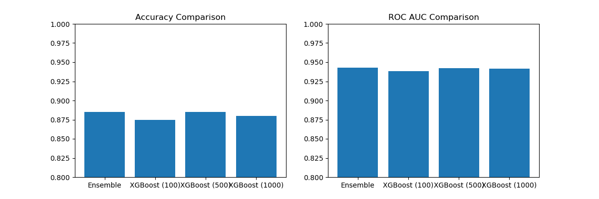
The plot may look like the following:

In this example, we generate a synthetic binary classification dataset and train a single XGBoost model with a high number of boosting rounds (1000). We then use the iteration_range parameter in the predict_proba() method to obtain predictions at different boosting levels: 100 (early stopping), 500 (moderate fit), and 1000 (potential overfit).
Next, we combine the predictions from each level by averaging the predicted probabilities. We evaluate the performance of the ensemble predictions and the individual models at each boosting level using accuracy and ROC AUC as the metrics.
Finally, we visualize the performance comparison using side-by-side bar plots, which show the accuracy and ROC AUC of the ensemble and the individual XGBoost models at each boosting level.
By creating a horizontal ensemble of XGBoost models with different boosting levels, we can potentially leverage the predictions from various stages of the boosting process to improve overall performance. This approach may help balance between underfitting and overfitting by combining models with different levels of complexity.
Note that the performance gains from this horizontal ensembling technique may vary depending on the specific dataset and problem at hand. It’s essential to evaluate the ensemble approach against individual models to determine if it provides a significant benefit for your particular use case.
