This example demonstrates how to use XGBoost with scikit-learn’s MultiOutputRegressor for multi-step univariate time series forecasting, where we predict multiple future time steps based on a single input time series.
We’ll cover data preparation, model initialization, training, and making predictions using a synthetic dataset, highlighting the effectiveness of this approach for predicting multiple future time steps.
# XGBoosting.com
# Multi-step Univariate Time Series Forecasting with XGBoost and MultiOutputRegressor
import numpy as np
import pandas as pd
from xgboost import XGBRegressor
from sklearn.multioutput import MultiOutputRegressor
from sklearn.metrics import mean_squared_error
import matplotlib.pyplot as plt

# Generate a synthetic univariate time series dataset
series = np.sin(0.1 * np.arange(200)) + np.random.randn(200) * 0.1

# Prepare data for supervised learning
df = pd.DataFrame({'series': series})
for i in range(1, 6):
    df[f'lag_{i}'] = df['series'].shift(i)
df = df.dropna()

# Define a function to create input features and target variables for multi-step forecasting
def create_dataset(data, n_steps_in, n_steps_out):
    X, y = [], []
    for i in range(len(data) - n_steps_in - n_steps_out + 1):
        X.append(data[i : i + n_steps_in])
        y.append(data[i + n_steps_in : i + n_steps_in + n_steps_out])
    return np.array(X), np.array(y)

n_steps_in, n_steps_out = 5, 3
X, y = create_dataset(df['series'].values, n_steps_in, n_steps_out)

# Chronological split of data into train and test sets
split_index = int(len(X) * 0.8)
X_train, X_test = X[:split_index], X[split_index:]
y_train, y_test = y[:split_index], y[split_index:]

# Initialize an XGBRegressor model wrapped in a MultiOutputRegressor
base_model = XGBRegressor(n_estimators=100, learning_rate=0.1, random_state=42)
model = MultiOutputRegressor(base_model)

# Fit the model on the training data
model.fit(X_train, y_train)

# Make multi-step predictions on the test set
y_pred = model.predict(X_test)

# Evaluate the model's performance
mse = mean_squared_error(y_test, y_pred)
print(f"Mean Squared Error: {mse:.4f}")

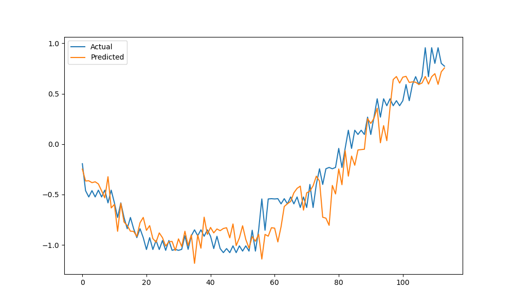
# Visualize the actual vs. predicted values for the test set
plt.figure(figsize=(10, 6))
plt.plot(y_test.flatten(), label='Actual')
plt.plot(y_pred.flatten(), label='Predicted')
plt.legend()
plt.show()
The plot may look as follows:

This example showcases how to use XGBoost with MultiOutputRegressor for multi-step univariate time series forecasting.
The key steps include:
- Generate a synthetic univariate time series dataset using a sine wave with added noise.
- Prepare the data for supervised learning by creating lagged features.
- Define a function
create_dataset()to generate input features and target variables for multi-step forecasting. - Split the data chronologically into train and test sets.
- Initialize an
XGBRegressormodel wrapped in aMultiOutputRegressor. - Fit the model on the training data.
- Make multi-step predictions on the test set.
- Evaluate the model’s performance using Mean Squared Error (MSE).
- Visualize the actual vs. predicted values for the test set.
By using XGBoost with MultiOutputRegressor, you can effectively predict multiple future time steps in a univariate time series. This approach can be adapted to various real-world forecasting tasks by adjusting the data preparation, hyperparameters, and the number of input and output steps.
