The tree_method parameter in XGBoost controls the algorithm used for constructing trees during the training process.
Choosing the right tree_method can impact both the training speed and the model’s performance.
This example demonstrates how to compare different tree_method options using a benchmark dataset to help you select the most appropriate algorithm for your use case.
import xgboost as xgb
import numpy as np
import time
from sklearn.datasets import make_classification
from sklearn.metrics import accuracy_score
import matplotlib.pyplot as plt

# Create a synthetic dataset
X, y = make_classification(n_samples=10000, n_classes=2, n_features=20, n_informative=10, random_state=42)

# Define tree_method options to compare
tree_methods = ['auto', 'exact', 'approx', 'hist']

# Set up XGBoost classifier
model = xgb.XGBClassifier(n_estimators=100, learning_rate=0.1, random_state=42)

# Dictionary to store results
results = {'tree_method': [], 'train_time': [], 'accuracy': []}

# Loop through tree_method options
for method in tree_methods:
    model.set_params(tree_method=method)

    start_time = time.time()
    model.fit(X, y)
    end_time = time.time()

    train_time = end_time - start_time
    accuracy = accuracy_score(y, model.predict(X))

    results['tree_method'].append(method)
    results['train_time'].append(train_time)
    results['accuracy'].append(accuracy)

# Print results table
print("{:<10} {:<15} {:<10}".format('Method', 'Train Time (s)', 'Accuracy'))
print("-"*35)
for i in range(len(tree_methods)):
    print("{:<10} {:<15.2f} {:<10.4f}".format(results['tree_method'][i], results['train_time'][i], results['accuracy'][i]))

# Plot training time comparison
plt.figure(figsize=(8, 6))
plt.bar(results['tree_method'], results['train_time'])
plt.title('Training Time Comparison')
plt.xlabel('Tree Method')
plt.ylabel('Training Time (s)')
plt.show()

# Plot accuracy comparison
plt.figure(figsize=(8, 6))
plt.bar(results['tree_method'], results['accuracy'])
plt.title('Accuracy Comparison')
plt.xlabel('Tree Method')
plt.ylabel('Accuracy')
plt.ylim(0.9, 1.0)
plt.show()
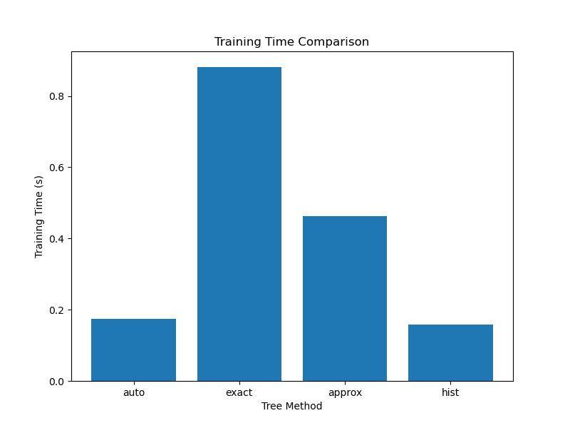
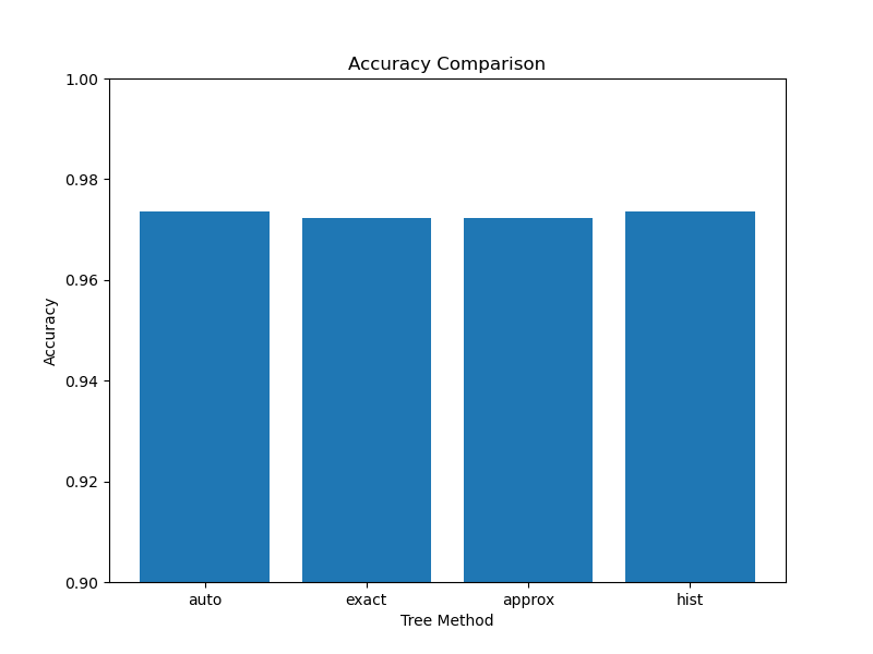
The resulting plots may look as follows:


In this example, we create a synthetic binary classification dataset using scikit-learn’s make_classification function. We then define a list of tree_method options to compare, including ‘auto’, ’exact’, ‘approx’, and ‘hist’.
We set up an instance of the XGBClassifier with default hyperparameters and create a dictionary called results to store the training time and accuracy for each tree_method.
We loop through the tree_method options, setting the tree_method parameter of the classifier using model.set_params(). For each option, we record the start time, train the classifier on the dataset, record the end time, and calculate the training time. We also evaluate the classifier’s accuracy on the dataset using accuracy_score(). The training time and accuracy are stored in the results dictionary.
After the loop, we print a table comparing the training time and accuracy for each tree_method. We then plot two bar charts using matplotlib to visualize the comparison of training times and accuracies.
The results can help you understand the trade-offs between training speed and model performance for different tree_method options. In general, the ’exact’ method is the slowest but most accurate, while the ‘hist’ method is the fastest but may have slightly lower accuracy. The ‘auto’ method automatically selects the best algorithm based on the dataset and system configuration, while ‘approx’ uses an approximation algorithm to speed up training.
Based on the results and your specific requirements (e.g., training time constraints or accuracy targets), you can choose the most appropriate tree_method for your use case. If training speed is a priority and you can afford a small accuracy trade-off, ‘hist’ or ‘approx’ might be good choices. If accuracy is the top concern and training time is not a limiting factor, ’exact’ would be the preferred option.
