
The num_parallel_tree parameter in XGBoost controls the number of parallel trees constructed during each iteration.
By increasing this value, you can potentially improve the training speed and model performance. However, the optimal value depends on your specific dataset and problem.
This example demonstrates how to find the best num_parallel_tree value using grid search with cross-validation.
import xgboost as xgb
import numpy as np
from sklearn.datasets import make_classification
from sklearn.model_selection import GridSearchCV, StratifiedKFold
from sklearn.metrics import accuracy_score

# Create a synthetic dataset
X, y = make_classification(n_samples=1000, n_classes=2, n_features=20, n_informative=10, random_state=42)

# Configure cross-validation
cv = StratifiedKFold(n_splits=5, shuffle=True, random_state=42)

# Define hyperparameter grid
param_grid = {
    'num_parallel_tree': [1, 2, 4, 8]
}

# Set up XGBoost classifier
model = xgb.XGBClassifier(n_estimators=100, learning_rate=0.1, random_state=42)

# Perform grid search
grid_search = GridSearchCV(estimator=model, param_grid=param_grid, cv=cv, scoring='accuracy', n_jobs=-1, verbose=1)
grid_search.fit(X, y)

# Get results
print(f"Best num_parallel_tree: {grid_search.best_params_['num_parallel_tree']}")
print(f"Best CV accuracy: {grid_search.best_score_:.4f}")

# Plot num_parallel_tree vs. accuracy
import matplotlib.pyplot as plt
results = grid_search.cv_results_

plt.figure(figsize=(10, 6))
plt.plot(param_grid['num_parallel_tree'], results['mean_test_score'], marker='o', linestyle='-', color='b')
plt.fill_between(param_grid['num_parallel_tree'], results['mean_test_score'] - results['std_test_score'],
                 results['mean_test_score'] + results['std_test_score'], alpha=0.1, color='b')
plt.title('Num Parallel Tree vs. Accuracy')
plt.xlabel('Num Parallel Tree')
plt.ylabel('CV Average Accuracy')
plt.grid(True)
plt.show()

# Train a final model with the best num_parallel_tree value
best_num_parallel_tree = grid_search.best_params_['num_parallel_tree']
final_model = xgb.XGBClassifier(n_estimators=100, learning_rate=0.1, num_parallel_tree=best_num_parallel_tree, random_state=42)
final_model.fit(X, y)
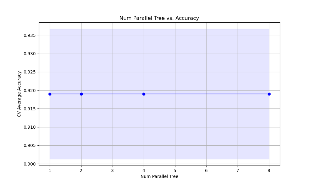
The resulting plot may look as follows:
In this example, we create a synthetic binary classification dataset using scikit-learn’s make_classification function. We then set up a StratifiedKFold cross-validation object to ensure that the class distribution is preserved in each fold.
We define a hyperparameter grid param_grid that specifies the values of num_parallel_tree we want to test. In this case, we consider values of 1, 2, 4, and 8.
We create an instance of the XGBClassifier with some basic hyperparameters set, such as n_estimators and learning_rate. We then perform the grid search using GridSearchCV, providing the model, parameter grid, cross-validation object, scoring metric (accuracy), and the number of CPU cores to use for parallel computation.
After fitting the grid search object with grid_search.fit(X, y), we can access the best num_parallel_tree value and the corresponding best cross-validation accuracy using grid_search.best_params_ and grid_search.best_score_, respectively.
We plot the relationship between the num_parallel_tree values and the cross-validation average accuracy scores using matplotlib. We retrieve the results from grid_search.cv_results_ and plot the mean accuracy scores along with the standard deviation as error bars. This visualization helps us understand how the choice of num_parallel_tree affects the model’s performance.
Finally, we train a final model using the best num_parallel_tree value found during the grid search. This model can be used for making predictions on new data.
By tuning the num_parallel_tree hyperparameter using grid search with cross-validation, we can find the optimal value that balances training speed and model performance for our specific problem. Keep in mind that the best value may vary depending on the dataset and the computational resources available.