
The learning_rate parameter in XGBoost controls the step size at each boosting iteration.
It determines the contribution of each tree to the final prediction.
An alias for the learning_rate parameter is eta.
Smaller learning rates generally lead to better generalization but require more boosting rounds to achieve the same level of performance. Larger learning rates can converge faster but may result in suboptimal solutions.
This example demonstrates how to tune the learning_rate hyperparameter using grid search with cross-validation to find the optimal value that balances model performance and training time.
import xgboost as xgb
import numpy as np
from sklearn.datasets import make_regression
from sklearn.model_selection import GridSearchCV, KFold
from sklearn.metrics import mean_squared_error

# Create a synthetic dataset
X, y = make_regression(n_samples=1000, n_features=20, noise=0.1, random_state=42)

# Configure cross-validation
cv = KFold(n_splits=5, shuffle=True, random_state=42)

# Define hyperparameter grid
param_grid = {
    'learning_rate': [0.01, 0.05, 0.1, 0.2, 0.3]
}

# Set up XGBoost regressor
model = xgb.XGBRegressor(n_estimators=100, subsample=0.8, colsample_bytree=0.8, random_state=42)

# Perform grid search
grid_search = GridSearchCV(estimator=model, param_grid=param_grid, cv=cv, scoring='neg_mean_squared_error', n_jobs=-1, verbose=1)
grid_search.fit(X, y)

# Get results
print(f"Best learning_rate: {grid_search.best_params_['learning_rate']}")
print(f"Best CV MSE: {-grid_search.best_score_:.4f}")

# Plot learning_rate vs. MSE
import matplotlib.pyplot as plt
results = grid_search.cv_results_

plt.figure(figsize=(10, 6))
plt.plot(param_grid['learning_rate'], -results['mean_test_score'], marker='o', linestyle='-', color='b')
plt.fill_between(param_grid['learning_rate'], -results['mean_test_score'] - results['std_test_score'],
                 -results['mean_test_score'] + results['std_test_score'], alpha=0.1, color='b')
plt.xscale('log')
plt.title('Learning Rate vs. MSE')
plt.xlabel('Learning Rate (log scale)')
plt.ylabel('CV Average MSE')
plt.grid(True)
plt.show()
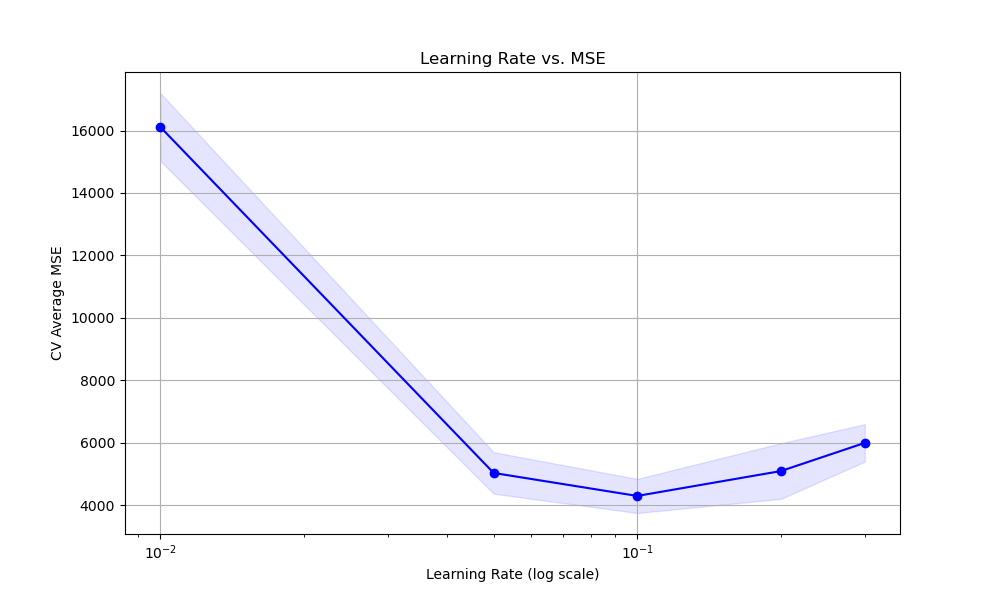
The resulting plot may look as follows:
In this example, we create a synthetic regression dataset using scikit-learn’s make_regression function. We then set up a KFold cross-validation object to split the data into training and validation sets.
We define a hyperparameter grid param_grid that specifies the range of learning_rate values we want to test. Here, we consider values of 0.01, 0.05, 0.1, 0.2, and 0.3.
We create an instance of the XGBRegressor with some basic hyperparameters set, such as n_estimators, subsample, and colsample_bytree. We then perform the grid search using GridSearchCV, providing the model, parameter grid, cross-validation object, scoring metric (negative mean squared error), and the number of CPU cores to use for parallel computation.
After fitting the grid search object with grid_search.fit(X, y), we can access the best learning_rate value and the corresponding best cross-validation mean squared error (MSE) using grid_search.best_params_ and grid_search.best_score_, respectively.
Finally, we plot the relationship between the learning_rate values and the cross-validation average MSE scores using matplotlib. We retrieve the results from grid_search.cv_results_ and plot the mean MSE scores along with the standard deviation as error bars. We use a logarithmic scale for the x-axis to better visualize the range of learning rates. This visualization helps us understand how the choice of learning_rate affects the model’s performance and guides us in selecting an appropriate value.
By tuning the learning_rate hyperparameter using grid search with cross-validation, we can find the optimal value that balances the model’s performance and training time. This helps ensure that the model converges to a good solution while avoiding overfitting or underfitting.