Explain XGBoost Predictions with SHAP

SHAP (SHapley Additive exPlanations) is a game-theoretic approach to explain the output of machine learning models.

It assigns each feature an importance value for a particular prediction, allowing you to interpret the model’s behavior on both global and local levels.

This example demonstrates how to use SHAP to interpret XGBoost predictions on a synthetic binary classification dataset.

First, install the shap library using our preferred Python package manager, such as pip:

pip install shap

Then, use the following code to generate a synthetic dataset, train an XGBoost model, and explain its predictions using SHAP:

from sklearn.datasets import make_classification
from sklearn.model_selection import train_test_split
from xgboost import XGBClassifier
import shap

# Generate a synthetic binary classification dataset
X, y = make_classification(n_samples=1000, n_features=10, n_informative=5, n_redundant=5, random_state=42)

# Split the data into train and test sets
X_train, X_test, y_train, y_test = train_test_split(X, y, test_size=0.2, random_state=42)

# Train an XGBoost classifier
model = XGBClassifier(n_estimators=100, random_state=42)
model.fit(X_train, y_train)

# Initialize a SHAP explainer with the trained model
explainer = shap.TreeExplainer(model)

# Calculate SHAP values for the test set
shap_values = explainer.shap_values(X_test)

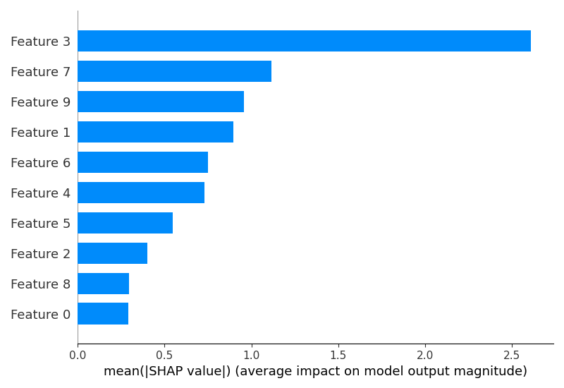
# Visualize global feature importances
shap.summary_plot(shap_values, X_test, plot_type="bar")

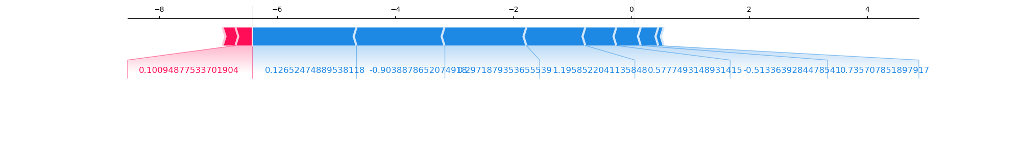
# Interpret an individual prediction
idx = 42
shap.force_plot(explainer.expected_value, shap_values[idx,:], X_test[idx,:], matplotlib=True)

The generated plots may look as follows:

In this example:

1. We generate a synthetic binary classification dataset using scikit-learn’s make_classification function with 1000 samples and 10 features, 5 of which are informative and 5 are redundant.

2. We split the dataset into training and test sets and train an XGBoost classifier on the training data.

3. We initialize a SHAP TreeExplainer with the trained XGBoost model. This explainer is specifically designed for tree-based models like XGBoost.

4. We calculate SHAP values for the test set using the shap_values method of the explainer. These values represent the feature importances for each instance in the test set.

5. We visualize the global feature importances using SHAP’s summary_plot function with plot_type="bar". This plot shows the mean absolute SHAP values for each feature, providing an overview of the most influential features in the model.

6. To interpret an individual prediction, we select a random instance from the test set (instance_idx = 42) and use SHAP’s force_plot function. This plot shows how each feature contributes to the model’s prediction for this specific instance, with positive values pushing the prediction towards the positive class and negative values pushing it towards the negative class.

SHAP provides a powerful way to interpret XGBoost models by quantifying the impact of each feature on the model’s predictions. The summary_plot gives a global view of feature importances, while the force_plot allows you to understand the factors driving a specific prediction. By combining these insights, you can gain a deeper understanding of your model’s behavior and make more informed decisions based on its predictions.