XGBoost Training Time of Tree Method vs Boosting Rounds

When training XGBoost models, the tree_method parameter plays a crucial role in determining the algorithm used for building trees.

Different tree methods can have varying impacts on training time and model performance. In this example, we’ll compare the training times of four commonly used tree methods: ’exact’, ‘approx’, and ‘hist’, while also varying the number of estimators.

We’ll use a synthetic dataset for binary classification and measure the training time for each combination of tree_method and n_estimators.

Finally, we’ll visualize the results as line plots to help us understand the relationship between these parameters and training time.

import time
import numpy as np
import pandas as pd
from sklearn.datasets import make_classification
from xgboost import XGBClassifier
import matplotlib.pyplot as plt

# Generate a synthetic dataset for binary classification
X, y = make_classification(n_samples=10000, n_features=20, n_informative=10, n_redundant=5, random_state=42)

# Define the range of tree_method values and n_estimators to test
tree_methods = ['exact', 'approx', 'hist', 'gpu_hist']
estimators_range = [10, 50, 100, 200, 300, 400, 500]

# Initialize a DataFrame to store the results
results_df = pd.DataFrame(columns=['tree_method', 'estimators', 'training_time'])

# Iterate over the tree_method values and n_estimators
for method in tree_methods:
    for estimators in estimators_range:
        # Initialize an XGBClassifier with the specified parameters
        model = XGBClassifier(tree_method=method, n_estimators=estimators, random_state=42)

        # Train the model and record the training time
        start_time = time.perf_counter()
        model.fit(X, y)
        end_time = time.perf_counter()
        training_time = end_time - start_time

        result = pd.DataFrame([{
            'tree_method': method,
            'estimators': estimators,
            'training_time': training_time
        }])

        # Report progress
        print(result)

        # Append the results to the DataFrame
        results_df = pd.concat([results_df, result], ignore_index=True)

# Pivot the DataFrame to create a matrix suitable for plotting
plot_df = results_df.pivot(index='estimators', columns='tree_method', values='training_time')

# Create a line plot
plt.figure(figsize=(10, 6))
for method in tree_methods:
    plt.plot(plot_df.index, plot_df[method], marker='o', label=method)

plt.xlabel('Number of Estimators')
plt.ylabel('Training Time (seconds)')
plt.title('XGBoost Training Time vs. Number of Estimators and Tree Method')
plt.legend(title='Tree Method')
plt.grid(True)
plt.xticks(estimators_range)
plt.show()

The resulting plot will display the training times for each tree_method as the number of estimators increases.

This allows us to compare the performance of different tree methods and understand how they scale with the number of estimators.

The plot may look something like the following:

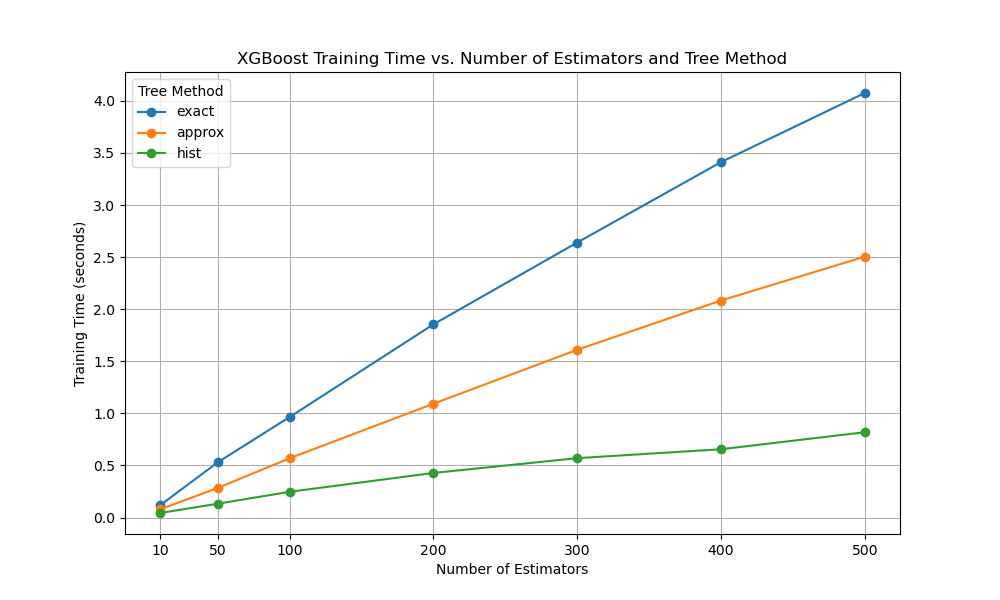
Plot of xgboost tree_method vs n_estimators

By visualizing the results, we can make informed decisions when selecting the appropriate tree_method for our XGBoost models, considering both training time and model performance. Keep in mind that the optimal choice of tree_method may also depend on the specific characteristics of your dataset and the computational resources available.

Note: The ‘gpu_hist’ method requires an XGBoost installation with GPU support, so make sure to set up the appropriate environment if you want to include this method in your comparison.

See Also