
Ensemble methods can be used to obtain stable predictions by combining multiple models trained with different random seeds.
In this example, we demonstrate how to create an ensemble of XGBoost models for regression tasks, where the final prediction is the mean or mean and standard deviation of the individual model predictions.
By using an ensemble of XGBoost models with different random seeds, we can mitigate the variability that arises from the randomness in the training process.
This results in more stable and consistent predictions for a fixed model configuration.
from sklearn.datasets import make_regression
from sklearn.model_selection import train_test_split
from xgboost import XGBRegressor
import numpy as np
import matplotlib.pyplot as plt

# Generate a synthetic regression dataset
X, y = make_regression(n_samples=1000, n_features=10, noise=0.1, random_state=42)
X_train, X_test, y_train, y_test = train_test_split(X, y, test_size=0.1, random_state=42)

# Define a function to create and train an XGBoost model with a specified random seed
def create_model(seed):
    model = XGBRegressor(n_estimators=100, subsample=0.8, learning_rate=0.01, random_state=seed)
    model.fit(X_train, y_train)
    return model

# Create multiple XGBoost models with different random seeds
n_models = 5
seeds = range(1, (n_models+1))
models = [create_model(seed) for seed in seeds]

# Make predictions using each model in the ensemble
y_preds = [model.predict(X_test) for model in models]

# Calculate the mean and standard deviation of the ensemble predictions
ensemble_mean = np.mean(y_preds, axis=0)
ensemble_std = np.std(y_preds, axis=0)

# Make a single prediction for reference
n = 5
yhats = [model.predict([X_test[n]]) for model in models]
print(f'Expected {y_test[n]}')
print(f'Predicted: {np.mean(yhats):.3f} +/- ({np.std(yhats):.3f})')
print(f'From: {[yhat[0] for yhat in yhats]}')

# Visualize the individual model predictions and the ensemble prediction
plt.figure(figsize=(8, 6))
for i, y_pred in enumerate(y_preds):
    plt.scatter(y_test, y_pred, label=f'Model {i+1}', alpha=0.7)
plt.scatter(y_test, ensemble_mean, label='Ensemble (Mean)', color='black', s=100, marker='x')
plt.errorbar(y_test, ensemble_mean, yerr=ensemble_std, fmt='none', ecolor='black', capsize=5)
plt.xlabel('True Values')
plt.ylabel('Predicted Values')
plt.legend()
plt.show()
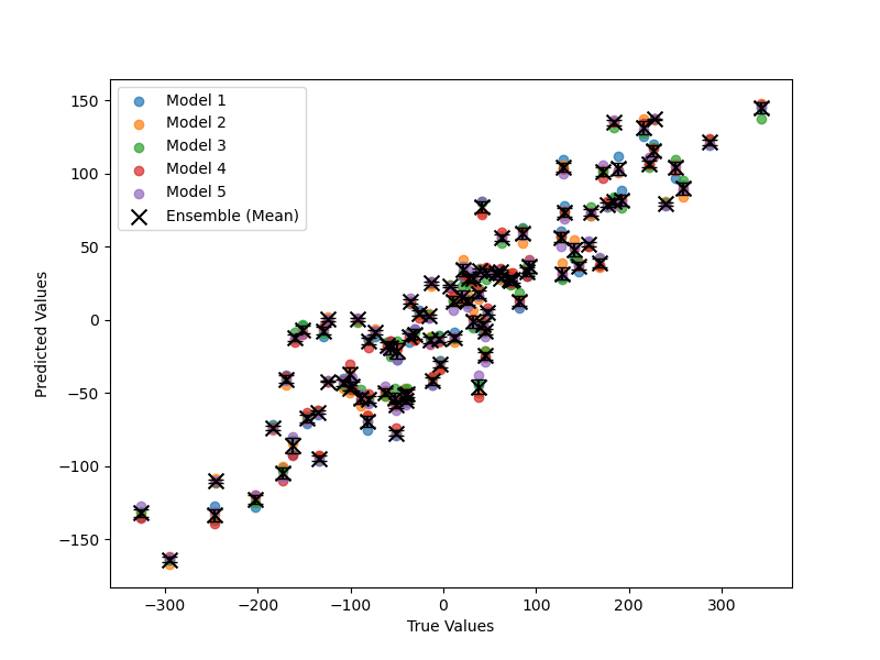
The plot may look like the following:
In this example, we generate a synthetic regression dataset using scikit-learn’s make_regression function and split it into train and test sets.
We define a function create_model that creates and trains an XGBoost model with a specified random seed. We then create multiple XGBoost models using different random seeds.
We make predictions using each model in the ensemble on the test set and store the predictions in the y_preds list.
Next, we calculate the mean and standard deviation of the ensemble predictions using NumPy’s mean and std functions, respectively.
Finally, we visualize the individual model predictions and the ensemble prediction using a scatter plot. The individual model predictions are plotted with different colors and labels, while the ensemble prediction (mean) is plotted as black cross markers. The standard deviation of the ensemble predictions is represented by error bars.
By creating an ensemble of XGBoost models with different random seeds, we can obtain more stable and consistent predictions compared to using a single model. The mean of the ensemble predictions provides a robust estimate, while the standard deviation quantifies the uncertainty in the predictions.