
Estimating prediction intervals is crucial for assessing the reliability of regression models.
While XGBoost is a powerful algorithm, it does not provide prediction intervals natively.
This example demonstrates how to estimate prediction intervals for XGBoost regression models using a diverse Monte Carlo ensemble approach.
By varying the random number seed and subsampling settings for each model in the ensemble, we create a more diverse set of predictions, which can lead to more robust prediction intervals.
from sklearn.datasets import make_regression
from sklearn.model_selection import train_test_split
from xgboost import XGBRegressor
import numpy as np
import matplotlib.pyplot as plt

# Generate a synthetic regression dataset
X, y = make_regression(n_samples=500, n_features=10, noise=0.1, random_state=42)

# Split data into train and test sets
X_train, X_test, y_train, y_test = train_test_split(X, y, test_size=0.2, random_state=42)

# Define a function to create a diverse Monte Carlo ensemble of XGBoost regressors
def diverse_monte_carlo_ensemble(X, y, n_models=100):
    models = []
    for i in range(n_models):
        # Vary the hyperparameters and subsampling settings for each model
        model = XGBRegressor(n_estimators=100, subsample=0.8, colsample_bytree=0.8,
                             max_depth=np.random.randint(3, 8), learning_rate=np.random.uniform(0.01, 0.2),
                             random_state=i)
        model.fit(X, y)
        models.append(model)
    return models

# Create a diverse Monte Carlo ensemble of XGBoost regressors
ensemble = diverse_monte_carlo_ensemble(X_train, y_train)

# Make predictions with each model in the ensemble
predictions = np.column_stack([model.predict(X_test) for model in ensemble])

# Compute the 2.5th and 97.5th percentiles of the predictions for a 95% prediction interval
lower = np.percentile(predictions, 2.5, axis=1)
upper = np.percentile(predictions, 97.5, axis=1)

# Visualize the true values vs. predictions with prediction intervals
plt.figure(figsize=(10, 7))
plt.scatter(y_test, predictions.mean(axis=1), alpha=0.5, label='Predictions')
plt.errorbar(y_test, predictions.mean(axis=1), yerr=[predictions.mean(axis=1) - lower, upper - predictions.mean(axis=1)],
             fmt='none', ecolor='gray', alpha=0.5, label='95% Prediction Interval')
plt.plot(y_test, y_test, '--', color='red', label='True Values')
plt.xlabel('True Values')
plt.ylabel('Predictions')
plt.title('XGBoost Regression Predictions with 95% Prediction Intervals (Diverse Monte Carlo Ensemble)')
plt.legend()
plt.tight_layout()
plt.show()
The plot may look like the following:
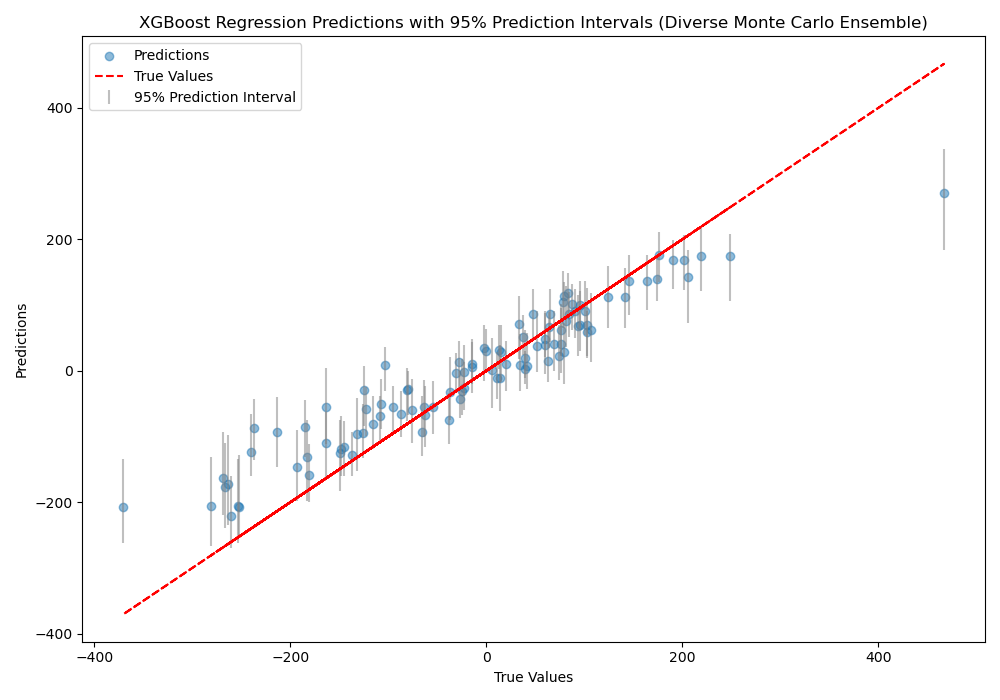
The code first generates a synthetic regression dataset and splits it into train and test sets. Next, we define a monte_carlo_ensemble function that creates n_models XGBoost regressors.
Each model in the ensemble is initialized with different random number seed and different hyperparameters settings:
subsample: The fraction of samples to be used for fitting each tree. Setting this to 0.8 means that each tree will be trained on a random 80% of the training data.colsample_bytree: The fraction of columns (features) to be used for fitting each tree. Setting this to 0.8 means that each tree will use a random 80% of the features.max_depth: The maximum depth of each tree. We randomly select a value between 3 and 7 for each model.learning_rate: The step size shrinkage used in updates to prevent overfitting. We randomly select a value between 0.01 and 0.2 for each model.
By varying these settings, we create a diverse ensemble of XGBoost regressors, where each model makes different decisions and produces different predictions. This diversity can lead to more robust prediction intervals that better capture the uncertainty of the model.
We then create a Monte Carlo ensemble of XGBoost regressors using the training data. Predictions are made with each model in the ensemble on the test data, and the results are stored in a matrix, where each column corresponds to a model’s predictions.
The 2.5th and 97.5th percentiles of the predictions are computed for each test instance to obtain the lower and upper bounds of the 95% prediction interval. Finally, we visualize the true values vs. the mean predictions with error bars representing the prediction intervals.
It’s important to note that while the Monte Carlo ensemble approach can provide an estimate of prediction intervals, it may not capture the full uncertainty of the model as effectively as bootstrap aggregation. The Monte Carlo method ideally only varies the random seed (although typically must vary a lot more to ensure a diversity of predictions), whereas bootstrap aggregation also varies the training data used for each model in the ensemble. As a result, the prediction intervals obtained from a Monte Carlo ensemble may be narrower and less representative of the true uncertainty compared to those obtained from bootstrap aggregation.