
Quantifying the uncertainty of individual predictions is crucial for assessing the reliability of regression models.
While XGBoost is a powerful algorithm for regression tasks, it does not natively provide prediction intervals.
This example demonstrates how to estimate prediction intervals for XGBoost regression models using the bootstrap aggregation (bagging) technique.
By creating an ensemble of XGBoost models trained on bootstrap samples of the data, we can gather predictions from each model and compute intervals based on the distribution of these predictions.
# XGBoosting.com
# Estimate Prediction Intervals for XGBoost Regression using Bootstrap Aggregation
from sklearn.datasets import make_regression
from sklearn.model_selection import train_test_split
from xgboost import XGBRegressor
import numpy as np
import matplotlib.pyplot as plt
# Generate a synthetic regression dataset
X, y = make_regression(n_samples=500, n_features=10, noise=0.1, random_state=42)
# Split data into train and test sets
X_train, X_test, y_train, y_test = train_test_split(X, y, test_size=0.2, random_state=42)
# Define a function to create bootstrap samples and train XGBoost models
def bootstrap_models(X, y, n_bootstraps=100):
models = []
for _ in range(n_bootstraps):
idx = np.random.choice(len(X), size=len(X), replace=True)
X_boot, y_boot = X[idx], y[idx]
model = XGBRegressor(n_estimators=100, random_state=42)
model.fit(X_boot, y_boot)
models.append(model)
return models
# Create an ensemble of XGBoost regressors using bootstrap aggregation
ensemble = bootstrap_models(X_train, y_train)
# Make predictions with each model in the ensemble
predictions = np.column_stack([model.predict(X_test) for model in ensemble])
# Compute the 2.5th and 97.5th percentiles of the predictions for a 95% prediction interval
lower = np.percentile(predictions, 2.5, axis=1)
upper = np.percentile(predictions, 97.5, axis=1)
# Visualize the true values vs. predictions with prediction intervals
plt.figure(figsize=(10, 7))
plt.scatter(y_test, predictions.mean(axis=1), alpha=0.5, label='Predictions')
plt.errorbar(y_test, predictions.mean(axis=1), yerr=[predictions.mean(axis=1) - lower, upper - predictions.mean(axis=1)],
fmt='none', ecolor='gray', alpha=0.5, label='95% Prediction Interval')
plt.plot(y_test, y_test, '--', color='red', label='True Values')
plt.xlabel('True Values')
plt.ylabel('Predictions')
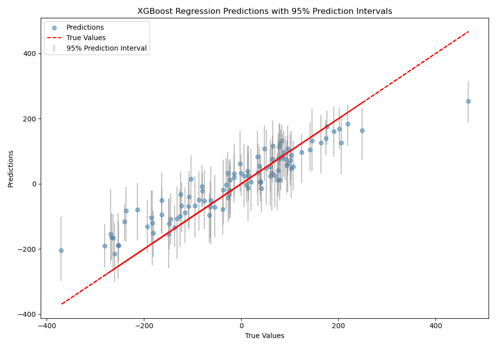
plt.title('XGBoost Regression Predictions with 95% Prediction Intervals')
plt.legend()
plt.tight_layout()
plt.show()
The plot may look like the following:
The code first generates a synthetic regression dataset using scikit-learn’s make_regression function. The data is then split into train and test sets.
Next, we define a bootstrap_models function that creates n_bootstraps samples of the training data with replacement, trains an XGBRegressor on each sample, and returns the list of trained models.
The bootstrap_models function is called with the training data to create an ensemble of XGBoost regressors.
We then make predictions with each model in the ensemble on the test data and store the predictions in a matrix, where each column corresponds to a model’s predictions.
The 2.5th and 97.5th percentiles of the predictions are computed for each test instance to obtain the lower and upper bounds of the 95% prediction interval.
Finally, we visualize the true values vs. the mean predictions with error bars representing the prediction intervals. This plot helps assess the quality of the predictions and the uncertainty captured by the intervals.
By using a bootstrap ensemble, we can estimate prediction intervals for XGBoost regression models, providing a measure of uncertainty for individual predictions.