
The n_jobs and nthread parameters in XGBoost control the number of parallel threads used during the training process, specifically during the tree construction phase.
Larger values allow for greater parallelization, potentially speeding up the training process.
The nthread parameter is preferred when using the native XGBoost API, while n_jobs is used in the scikit-learn API, conforming to the scikit-learn convention.
If both parameters are specified in a configuration, the nthread value will be used.
This example demonstrates how to use both parameters and confirms that they have the same effect on the model’s performance.
from sklearn.datasets import make_classification
from sklearn.model_selection import train_test_split
from xgboost import XGBClassifier
import time

# Generate a synthetic dataset
X, y = make_classification(n_samples=1000000, n_features=20, n_classes=2, random_state=42)

# Split the dataset into training and test sets
X_train, X_test, y_train, y_test = train_test_split(X, y, test_size=0.2, random_state=42)

# Create two XGBoost classifiers, one using "n_jobs" and the other using "nthread"
model_n_jobs = XGBClassifier(n_jobs=2, eval_metric='logloss')
model_nthread = XGBClassifier(nthread=2, eval_metric='logloss')

# Warm start
model_n_jobs.fit(X_train, y_train)
model_n_jobs = XGBClassifier(n_jobs=2, eval_metric='logloss')

# Train the n_jobs model on the training set
time_n_jobs_start = time.perf_counter()
model_n_jobs.fit(X_train, y_train)
time_n_jobs_end = time.perf_counter()
time_n_jobs_duration = time_n_jobs_end - time_n_jobs_start
print(f'n_jobs took {time_n_jobs_duration:.3f} seconds')

# Train the nthread model on the training set
time_nthread_start = time.perf_counter()
model_nthread.fit(X_train, y_train)
time_nthread_end = time.perf_counter()
time_nthread_duration = time_nthread_end - time_nthread_start
print(f'nthread took {time_nthread_duration:.3f} seconds')

# Make predictions on the test set
predictions_n_jobs = model_n_jobs.predict(X_test)
predictions_nthread = model_nthread.predict(X_test)

# Compare the results
assert (predictions_n_jobs == predictions_nthread).all()
The example below demonstrates the same functionality using the native XGBoost API with DMatrix:
import xgboost as xgb
from sklearn.datasets import make_classification
from sklearn.model_selection import train_test_split
import time

# Generate a synthetic dataset
X, y = make_classification(n_samples=1000000, n_features=20, n_classes=2, random_state=42)

# Split the dataset into training and test sets
X_train, X_test, y_train, y_test = train_test_split(X, y, test_size=0.2, random_state=42)

# Convert data to DMatrix
dtrain = xgb.DMatrix(X_train, label=y_train)
dtest = xgb.DMatrix(X_test, label=y_test)

# Set up parameters for XGBoost
params_n_jobs = {
    'objective': 'binary:logistic',
    'eval_metric': 'logloss',
    'n_jobs': 2,
}

params_nthread = {
    'objective': 'binary:logistic',
    'eval_metric': 'logloss',
    'nthread': 2,
}

# warm start
model_n_jobs = xgb.train(params_n_jobs, dtrain, num_boost_round=100)

# Train the n_jobs model on the training set
time_n_jobs_start = time.perf_counter()
model_n_jobs = xgb.train(params_n_jobs, dtrain, num_boost_round=100)
time_n_jobs_end = time.perf_counter()
time_n_jobs_duration = time_n_jobs_end - time_n_jobs_start
print(f'n_jobs took {time_n_jobs_duration:.3f} seconds')

# Train the nthread model on the training set
time_nthread_start = time.perf_counter()
model_nthread = xgb.train(params_nthread, dtrain, num_boost_round=100)
time_nthread_end = time.perf_counter()
time_nthread_duration = time_nthread_end - time_nthread_start
print(f'nthread took {time_nthread_duration:.3f} seconds')

# Make predictions on the test set
predictions_n_jobs = model_n_jobs.predict(dtest).round()
predictions_nthread = model_nthread.predict(dtest).round()

# Compare the results
assert (predictions_n_jobs == predictions_nthread).all()
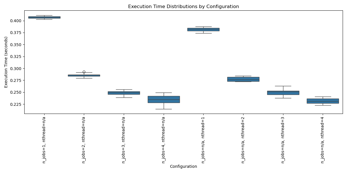
We can fit the same model many times with different values of n_jobs and again with same values of nthread.
The distribution of run times under each configuration show the same pattern of decreasing mean execution time as the number of n_jobs or nthread is increased.
import numpy as np
import xgboost as xgb
from sklearn.datasets import make_classification
from time import perf_counter
import pandas as pd
import seaborn as sns
import matplotlib.pyplot as plt

# Generate a dataset
X, y = make_classification(n_samples=10000, n_features=20, random_state=42)

# Parameter settings
n_jobs_values = [1, 2, 3, 4]
nthread_values = [1, 2, 3, 4]
repetitions = 10  # Number of repetitions for each setting

# Dictionary to store timing results
results = []

# Experiment loop 1
for n_jobs in n_jobs_values:
    times = []
    for _ in range(repetitions):
        clf = xgb.XGBClassifier(n_jobs=n_jobs, random_state=42)
        start_time = perf_counter()
        clf.fit(X, y)
        end_time = perf_counter()
        duration = end_time - start_time
        times.append(duration)
        # Report progress
        print(f'> n_jobs: {n_jobs} - {duration:3f} sec')

    # Record results
    results.append({
        'n_jobs': n_jobs,
        'nthread': 'n/a',
        'times': times
    })

# Experiment loop 2
for nthread in nthread_values:
    times = []
    for _ in range(repetitions):
        clf = xgb.XGBClassifier(nthread=nthread, random_state=42)
        start_time = perf_counter()
        clf.fit(X, y)
        end_time = perf_counter()
        duration = end_time - start_time
        times.append(duration)
        # Report progress
        print(f'> nthread: {nthread} - {duration:3f} sec')

    # Record results
    results.append({
        'n_jobs': 'n/a',
        'nthread': nthread,
        'times': times
    })

# Convert results to DataFrame for better visualization
result_df = pd.DataFrame(results)

# add config
result_df['config'] = result_df.apply(lambda row: f"n_jobs={row['n_jobs']}, nthread={row['nthread']}", axis=1)

# Printing summary statistics for each configuration
for index, row in result_df.iterrows():
    print(f"Configuration: {row['config']}")
    print(f"Mean: {np.mean(row['times']):.4f}, Std Dev: {np.std(row['times']):.4f}")
    print('-' * 40)

# Plotting
plt.figure(figsize=(12, 6))
sns.boxplot(x='config', y='times', data=result_df.explode('times'))
plt.xticks(rotation=90)
plt.title('Execution Time Distributions by Configuration')
plt.ylabel('Execution Time (seconds)')
plt.xlabel('Configuration')
plt.tight_layout()
plt.show()
Running the example creates a plot that may look as follows:
The choice between n_jobs and nthread ultimately depends on the API being used and personal preference. When working with XGBoost, it is recommended to use nthread when using the native XGBoost API and n_jobs when using the scikit-learn API.
It is important to note that the actual performance gains from increasing the number of parallel threads may vary depending on the dataset size, number of features, and the hardware being used. In some cases, especially with smaller datasets, the overhead of managing multiple threads may outweigh the benefits of parallelization.
Additionally, on Windows, the nthread parameter is not supported due to platform-specific limitations. In such cases, it is recommended to use the n_jobs parameter with the scikit-learn API.