
The n_jobs parameter in XGBoost controls the number of CPU cores used for parallel processing during model training.
By leveraging multiple cores, you can significantly reduce the training time, especially when working with large datasets.
An alias for the n_jobs parameter is nthread.
This example demonstrates how the n_jobs parameter affects the model fitting time.
import xgboost as xgb
import numpy as np
from sklearn.datasets import make_classification
import time
import matplotlib.pyplot as plt

# Generate a large synthetic dataset
X, y = make_classification(n_samples=100000, n_classes=2, n_features=20, n_informative=10, random_state=42)

# Define a function to measure model fitting time
def measure_fitting_time(n_jobs):
    start_time = time.perf_counter()
    model = xgb.XGBClassifier(n_estimators=100, n_jobs=n_jobs)
    model.fit(X, y)
    end_time = time.perf_counter()
    return end_time - start_time

# Test different n_jobs values
n_jobs_values = [-1, 1, 2, 3, 4, 5, 6, 7, 8]
fitting_times = []

for n_jobs in n_jobs_values:
    fitting_time = measure_fitting_time(n_jobs)
    fitting_times.append(fitting_time)
    print(f"n_jobs={n_jobs}, Fitting Time: {fitting_time:.2f} seconds")

# Plot the results
plt.figure(figsize=(8, 6))
plt.plot(n_jobs_values, fitting_times, marker='o', linestyle='-')
plt.title('n_jobs vs. Model Fitting Time')
plt.xlabel('n_jobs')
plt.ylabel('Fitting Time (seconds)')
plt.grid(True)
plt.xticks(n_jobs_values)
plt.show()
The resulting plot may look as follows:
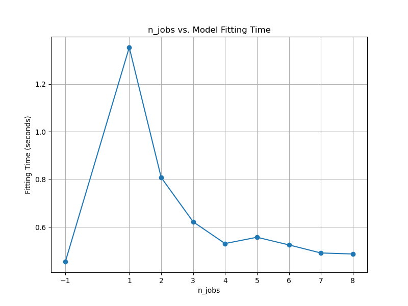
In this example, we generate a large synthetic dataset using scikit-learn’s make_classification function to simulate a realistic scenario where parallel processing can provide significant benefits.
We define a measure_fitting_time function that takes the n_jobs parameter as input, creates an XGBClassifier with the specified n_jobs value, fits the model on the dataset, and returns the model fitting time.
We then iterate over different n_jobs values (-1, 1, 2, 3, 4, 5, 6, 7, 8) and measure the model fitting time for each value. The -1 value indicates that all available CPU cores should be used.
After collecting the fitting times, we plot a graph using matplotlib to visualize the relationship between the n_jobs values and the corresponding model fitting times.
When you run this code, you will see the fitting times printed for each n_jobs value, and a graph will be displayed showing the impact of n_jobs on the model fitting time.
By setting n_jobs to a higher value, you can potentially reduce the model fitting time significantly, especially when working with large datasets. However, the actual speedup may vary depending on the number of available CPU cores and the specific dataset characteristics.
Note that using all available cores (n_jobs=-1) may not always be the optimal choice, as it can lead to high memory consumption. It’s recommended to experiment with different n_jobs values to find the best balance between training speed and resource utilization for your specific use case.