
The gamma parameter in XGBoost controls the minimum loss reduction required for a split to occur in a leaf node.
An alias for the gamma parameter is min_split_loss.
It acts as a regularization term that helps control the model’s complexity. Higher values of gamma make the algorithm more conservative, requiring a larger reduction in the loss function to create a new split. This can help prevent overfitting by limiting the model’s sensitivity to individual data points.
This example demonstrates how to tune the gamma hyperparameter using grid search with cross-validation to find the optimal value that balances model complexity and performance.
import xgboost as xgb
import numpy as np
from sklearn.datasets import make_classification
from sklearn.model_selection import GridSearchCV, StratifiedKFold
from sklearn.metrics import accuracy_score

# Create a synthetic dataset
X, y = make_classification(n_samples=1000, n_classes=3, n_features=20, n_informative=10, random_state=42)

# Configure cross-validation
cv = StratifiedKFold(n_splits=5, shuffle=True, random_state=42)

# Define hyperparameter grid
param_grid = {
    'gamma': [0, 0.1, 0.2, 0.3, 0.4, 0.5, 0.6, 0.7, 0.8, 0.9, 1.0]
}

# Set up XGBoost classifier
model = xgb.XGBClassifier(n_estimators=100, learning_rate=0.1, random_state=42)

# Perform grid search
grid_search = GridSearchCV(estimator=model, param_grid=param_grid, cv=cv, scoring='accuracy', n_jobs=-1, verbose=1)
grid_search.fit(X, y)

# Get results
print(f"Best gamma: {grid_search.best_params_['gamma']}")
print(f"Best CV accuracy: {grid_search.best_score_:.4f}")

# Plot gamma vs. accuracy
import matplotlib.pyplot as plt
results = grid_search.cv_results_

plt.figure(figsize=(10, 6))
plt.plot(param_grid['gamma'], results['mean_test_score'], marker='o', linestyle='-', color='b')
plt.fill_between(param_grid['gamma'], results['mean_test_score'] - results['std_test_score'],
                 results['mean_test_score'] + results['std_test_score'], alpha=0.1, color='b')
plt.title('Gamma vs. Accuracy')
plt.xlabel('Gamma')
plt.ylabel('CV Average Accuracy')
plt.grid(True)
plt.show()
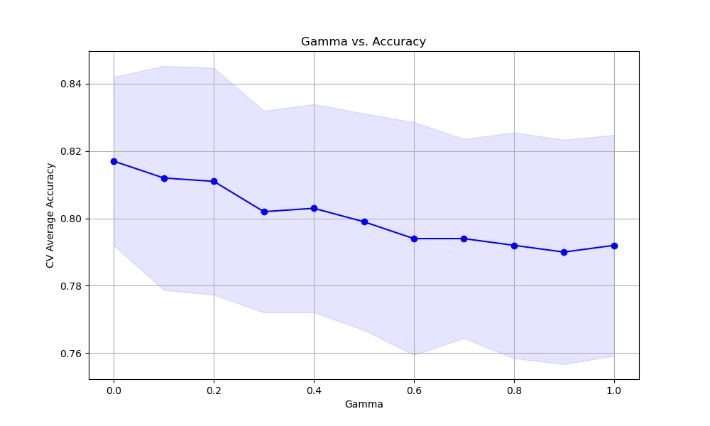
The resulting plot may look as follows:
In this example, we create a synthetic multiclass classification dataset using scikit-learn’s make_classification function. We then set up a StratifiedKFold cross-validation object to ensure that the class distribution is preserved in each fold.
We define a hyperparameter grid param_grid that specifies the range of gamma values we want to test. In this case, we consider values from 0 to 1.0 in increments of 0.1.
We create an instance of the XGBClassifier with some basic hyperparameters set, such as n_estimators and learning_rate. We then perform the grid search using GridSearchCV, providing the model, parameter grid, cross-validation object, scoring metric (accuracy), and the number of CPU cores to use for parallel computation.
After fitting the grid search object with grid_search.fit(X, y), we can access the best gamma value and the corresponding best cross-validation accuracy using grid_search.best_params_ and grid_search.best_score_, respectively.
Finally, we plot the relationship between the gamma values and the cross-validation average accuracy scores using matplotlib. We retrieve the results from grid_search.cv_results_ and plot the mean accuracy scores along with the standard deviation as error bars. This visualization helps us understand how the choice of gamma affects the model’s performance and guides us in selecting an appropriate value.
By tuning the gamma hyperparameter using grid search with cross-validation, we can find the optimal value that balances the model’s complexity and performance. This helps prevent overfitting and ensures that the model generalizes well to unseen data.