Explain XGBoost Predictions with LIME

Understanding why a machine learning model makes certain predictions can be as crucial as the predictions themselves.

LIME (Local Interpretable Model-agnostic Explanations) is a library that helps explain individual predictions made by any model, including XGBoost.

This example demonstrates how to use LIME to gain insights into the features driving a specific XGBoost prediction using a synthetic binary classification dataset.

Firstly, we must install the lime Python library using our preferred package manager, such as pip:

pip install lime

We can then use LIME explainability to understand our XGBoost model:

from sklearn.datasets import make_classification
from sklearn.model_selection import train_test_split
from xgboost import XGBClassifier
import lime
import lime.lime_tabular
import matplotlib.pyplot as plt

# Generate a synthetic binary classification dataset
X, y = make_classification(n_samples=1000, n_features=10, n_informative=5, n_redundant=5, random_state=42)

# Split the data into train and test sets
X_train, X_test, y_train, y_test = train_test_split(X, y, test_size=0.2, random_state=42)

# Train an XGBoost classifier
model = XGBClassifier(n_estimators=100, random_state=42)
model.fit(X_train, y_train)

# Select a random data point from the test set
instance_idx = 42
instance = X_test[instance_idx]

# Create a LIME explainer
explainer = lime.lime_tabular.LimeTabularExplainer(X_train, feature_names=[f'feature_{i}' for i in range(10)], class_names=['class_0', 'class_1'], discretize_continuous=True)

# Get the LIME explanation for the chosen instance
explanation = explainer.explain_instance(instance, model.predict_proba, num_features=10)

# Visualize the explanation
explanation.as_pyplot_figure()
plt.show()

The generated plot may look as follows:

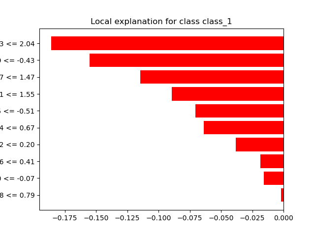
In this example:

1. We generate a synthetic binary classification dataset using scikit-learn’s make_classification function with 1000 samples and 10 features, 5 of which are informative and 5 are redundant.

2. We split the dataset into training and test sets and train an XGBoost classifier on the training data.

3. We select a random data point from the test set for which we want to explain the model’s prediction.

4. We create a LIME explainer by providing it with the training data, feature names, and class names. We set discretize_continuous=True to handle continuous features.

5. We generate a LIME explanation for the chosen instance by calling explain_instance with the instance, the model’s predict_proba function, and the desired number of features to include in the explanation.

6. Finally, we visualize the explanation using LIME’s as_pyplot_figure method, which shows the top features contributing to the model’s prediction for this specific instance.

LIME provides a helpful way to understand the factors driving an individual prediction made by an XGBoost model. By examining the features and their contributions, you can gain insights into what the model considers important for a particular instance. This can be valuable for model debugging, identifying potential biases, or explaining predictions to stakeholders.

Note that LIME explanations are local, meaning they are specific to the chosen instance and may not represent the model’s overall behavior. It’s essential to consider multiple instances and the global feature importances to get a comprehensive understanding of the model’s decision-making process.